Meet Quarto!

What is Quarto?

Quarto® is an open-source scientific and technical publishing system built on Pandoc .

It is designed to be a complete scientific and technical publishing system.
It can create dynamic content with multiple languages R, Julia, Python, and Observable.
It allows you to author documents as plain text markdown or executable notebooks.
You can author with scientific markdown, including equations, citations, crossrefs, figure panels, callouts, advanced layout, and more.
You can publish high-quality research using a single framework, Quarto.

Why Quarto?

Quarto provides a unified authoring framework for data science, combining your code, its results, and your prose. Quarto files are designed to be used in three ways:

For communicating to decision-makers, who want to focus on the conclusions and implications of your research and not the technicalities behind the analysis.
For collaborating with other researchers (including future you!).
As an environment in which to reproducible research where you can capture not only what you did, but also what you were thinking.

Quarto Basics

Installation

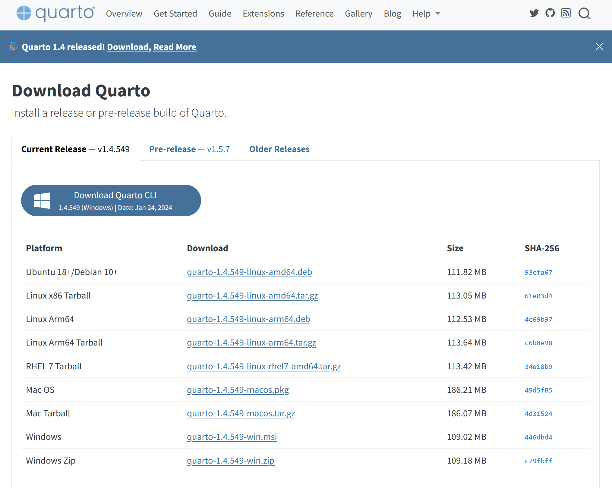
You can install Quarto from https://quarto.org/docs/download/.

Let Started with Quarto in RStudio

To get started, open RStudio and create a Quarto Document.

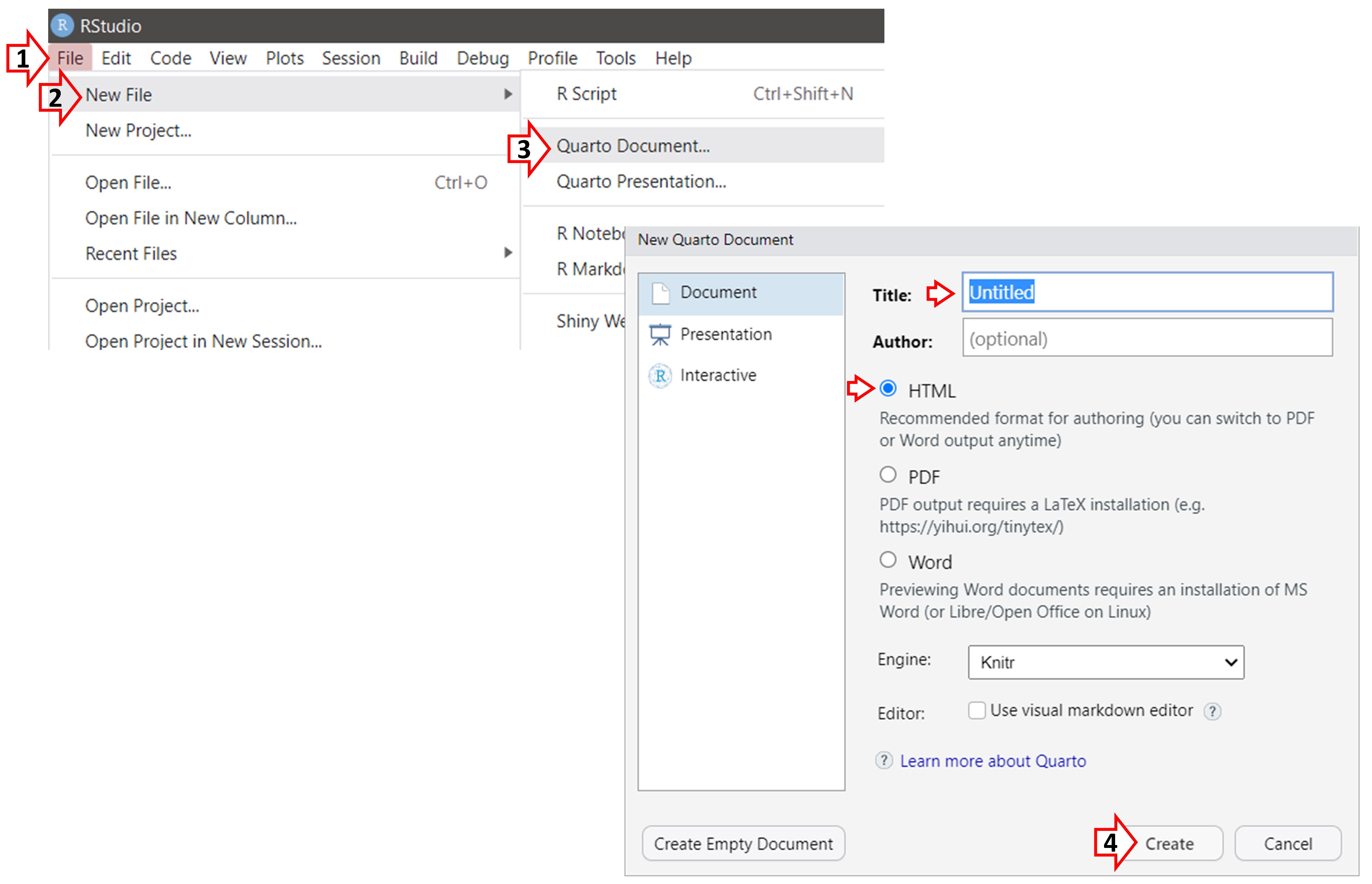
This will create a file with temporary content to help get you started.

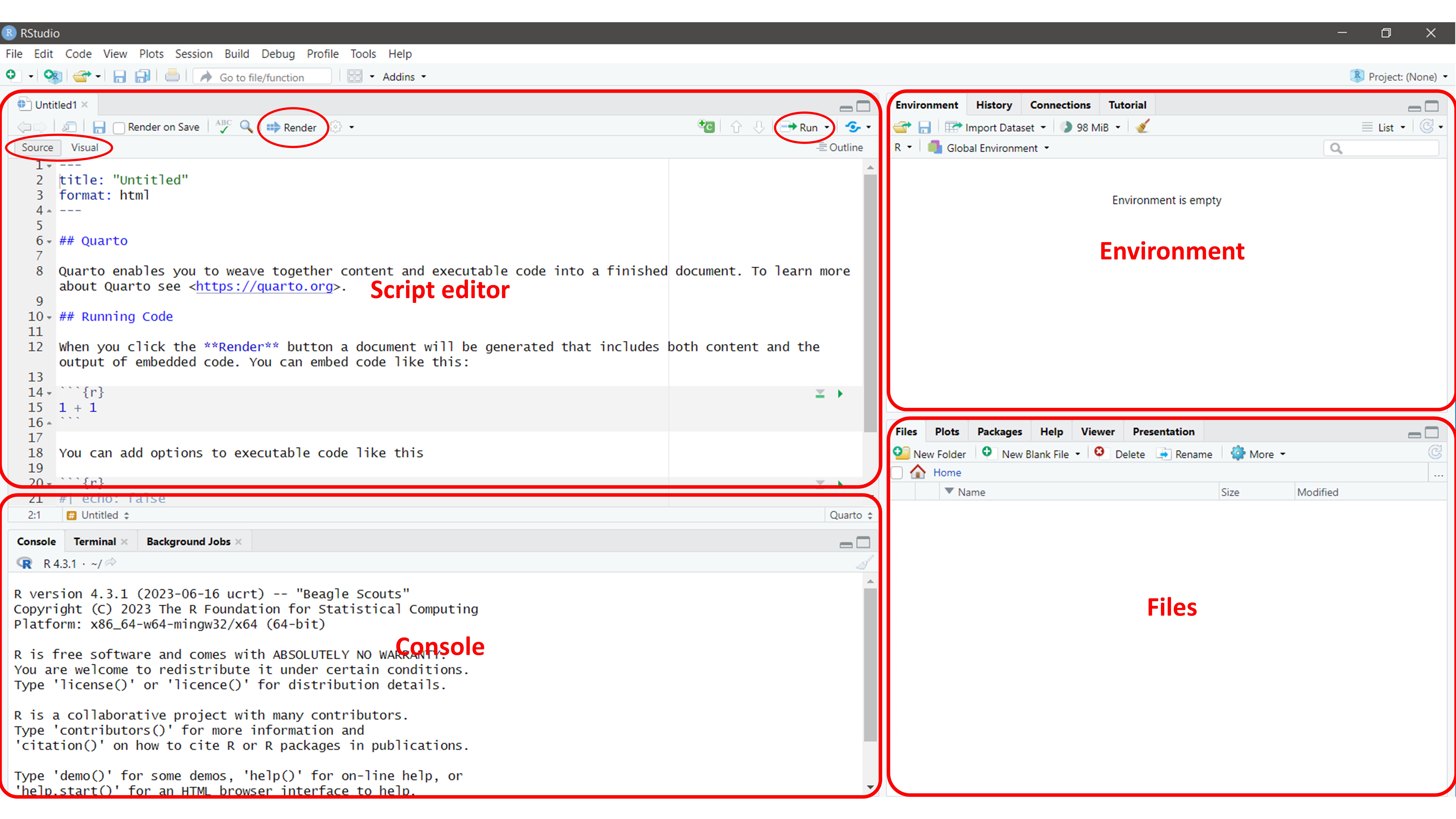
Figure 3: The **script editor** is where you write and edit your content. You can view the content using the **Source** view, which uses the raw syntax (used throughout this tutorial), or use the **Visual** view, which uses a point-and-click interface for formatting (similar to Microsoft Word).

All of the scripts provided below in this tutorial should be entered into the ‘Script Editor’. Clicking Render will generate the formatted document. You can also highlight code and click Run to execute specific lines of code.

The console is where you see the output of any statistical code. The environment panel displays information about the variables and objects in your current R session, while the files panel allows you to navigate your computer’s file system and manage your R projects.

Output Settings

Each quarto file starts with a set of code, called the YAML which is fenced within ---. The YAML specifics the metadata and document-wide settings.

For example, for a HTML document the YAML may be:

---
title: Introduction to Quarto
subtitle: My subtitle
author: Arun Mitra
date: last-modified
format: 
  html:
    self-contained: true
execute:
  echo: true
  warning: false
toc: true
number-sections: true
---

Explaination

format specifies the type of output file to generate. Here it is an HTML file.

self-contained: true specifies that the HTML file generated should be standalone file.

echo: true enables the printing of code (only output is displayed), unless otherwise specified.

warning: false disables the printing of warning messages.

toc: true specifies that the table of contents should be shown; automatically generated based on the headings.

number-sections: specifies that the numbering of the sections should be shown.

Formatting


# Heading 1

## Heading 2

### Heading 3

Bold text like **this** or __this__

Italicize text like *this* or _this_

Clickable link: <https://google.com>

[Hyperlink](google.com) 

-   Bullet point (nordered lists)
-   Hyphen, follwed by 'tab'

1.    Ordered list
2.    Number, period, then 'tab'

|            | Manual   | Table    |
|------------|----------|----------|
| Variable 1 | 11       | 21       |
| Variable 2 | 12       | 22       |
| Variable 3 | 12       | 23       |

Output

Heading 1

Heading 2

Heading 3

Bold text like this or this

Italicize text like this or this

Clickable link: https://google.com

Hyperlink

Bullet point (nordered lists)
Hyphen, follwed by ‘tab’

Ordered list
Number, period, then ‘tab’

	Var1	Var2
Observation 1	11	21
Observation 2	12	22
Observation 3	12	23

Code Chunks

Quarto can understand and run different programming languages, such as R and Python. This introduction focuses on R.

Code is specified within “code chunks”, which begin with ```{r} and end with ```

As an example, here’s a simple calculation using R; the syntax is shown along with the output automatically generated.

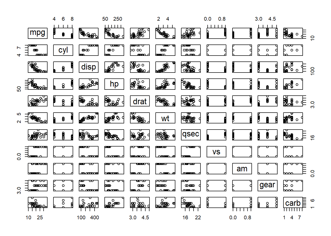
6 * 4

[1] 24

Here is one more example of creating a plot using an inbuilt dataset within R.

mtcars |> 
  plot()

Code Execution Options

There are a variety of options for how to handle the code and its output, called 'execution options'. These options are specified at the start of the code chunk, and begin with #|

For example, let us run the above code chunks with additional execution options:

Example 1:

Code:

#| echo: true
#| eval: false

6 * 4

Output:

6 * 4

Note that the code has been printed, but not evaluated (the answer, has not been printed).

Example 2:

Code:

#| echo: false
#| eval: true

mtcars |> 
  plot()

Output:

Example 3:

Additionally you can use the option code-fold to hide the code chunk, and reveal only when needed.

Code:

#| code-fold: true

# Load Packages
library(ggstatsplot)
library(palmerpenguins)
library(tidyverse)


# Load Data
penguins <- 
  data(penguins) |> 
  get()

# Remove missing values
penguins <- 
  penguins |> 
  drop_na()

# Create a plot

ggbetweenstats(
    data = penguins,
    x = species,
    y = bill_length_mm )

Output:

Code

# Load Packages
library(ggstatsplot)
library(palmerpenguins)
library(tidyverse)


# Load Data
penguins <- 
  data(penguins) |> 
  get()

# Remove missing values
penguins <- 
  penguins |> 
  drop_na()

# Create a plot

ggbetweenstats(
    data = penguins,
    x = species,
    y = bill_length_mm )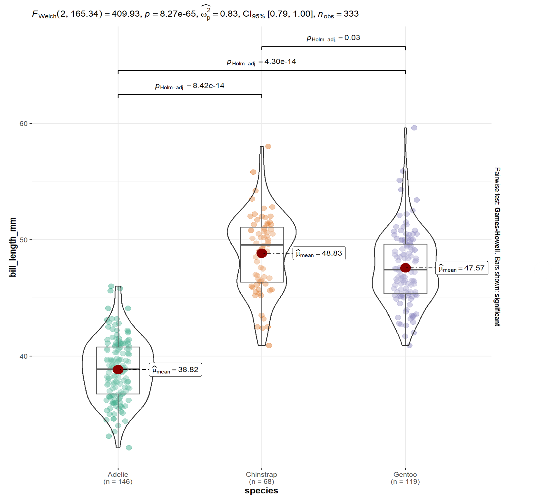

Note that the the output has been printed, however, if you want to see the code which produced this plot, you can click on the interactive Code button.

Few Additional features in Quarto!

Tabsets

Another way to organize a report is to present information in different tabs.

Similarly, as before, this is coded using ::: to denote the start and end of the information to be presented in tabs.

Level 3 headings (specified using ###) are used as the tab title and denote the start of each new tab.

Here a simple example:

Code:

::: {.panel-tabset}

### Panel 1
Content of panel 1

### Panel 2

```{r}
mtcars |> 
  plot()
```

:::

Content of panel 1

Layout

To create and work with columns, use ::: or ::::. Like brackets, these are used to indicate the start and end the content to be placed in columns.

Here’s an example of a Two Column Layout:

Content of column 1:

Bullet point 1
Bullet point 1
Bullet point 1

Content of column 2:

This can be an image as well:


::: columns
::: column
Content of column 1:

-   Bullet point 1
-   Bullet point 1
-   Bullet point 1
:::

::: column
Content of column 2:

This can be an image as well:

![](images/quarto_logo.png){width="50%"}
:::
:::

Call Out Blocks

Callouts are used to draw extra attention to certain concepts, or to more clearly indicate that certain content is supplemental or applicable to only some scenarios.

Callouts start with ::: {.callout-note}, then there’s the content, and it ends with :::.

There are five types of callouts:

`note`

:::{.callout-note}
This is a callout block of the type "note".
:::

Note

This is a callout block of the type “note”.

`warning`

:::{.callout-caution collapse="true"}
Callouts can be collapsible. 
:::

Warning

Callouts can be collapsible.

`important`

:::{.callout-important}
# My heading
The first heading used within the callout 
is used as the callout heading.
:::

My heading

The first heading used within the callout is used as the callout heading.

`tip`

:::{.callout-tip icon=false}
The icon can also be hidden, like this. 
:::

Tip

The icon can also be hidden, like this.

`caution`

:::{.callout-caution}
This is a caution callout
:::

Caution

This is a caution callout