library(sf)
library(tidyverse)
library(here)

districts <- read_rds(here("spatial_files", "india_district_sf.rds"))

ggplot(districts) +
  geom_sf(linewidth = 0.05, fill = "grey95", colour = "grey40") +
  theme_void()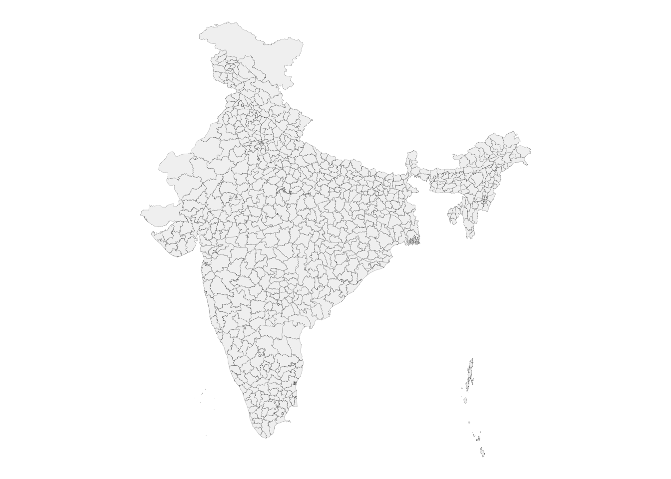
DMgtAsia · Session-II (1 of 2)
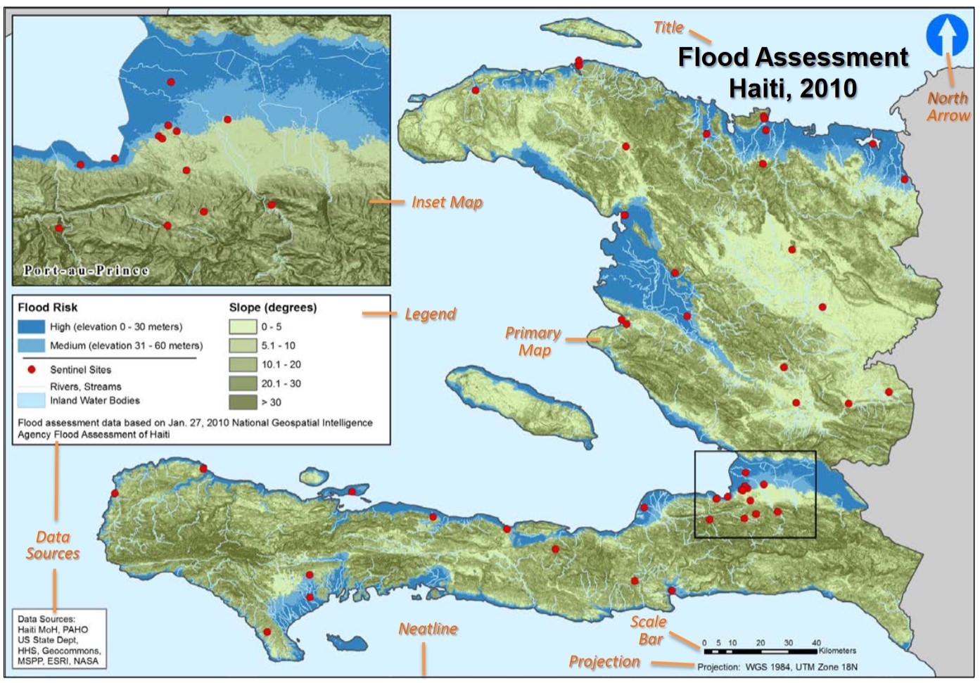
The map is to spatial analysis what the histogram is to ordinary EDA.
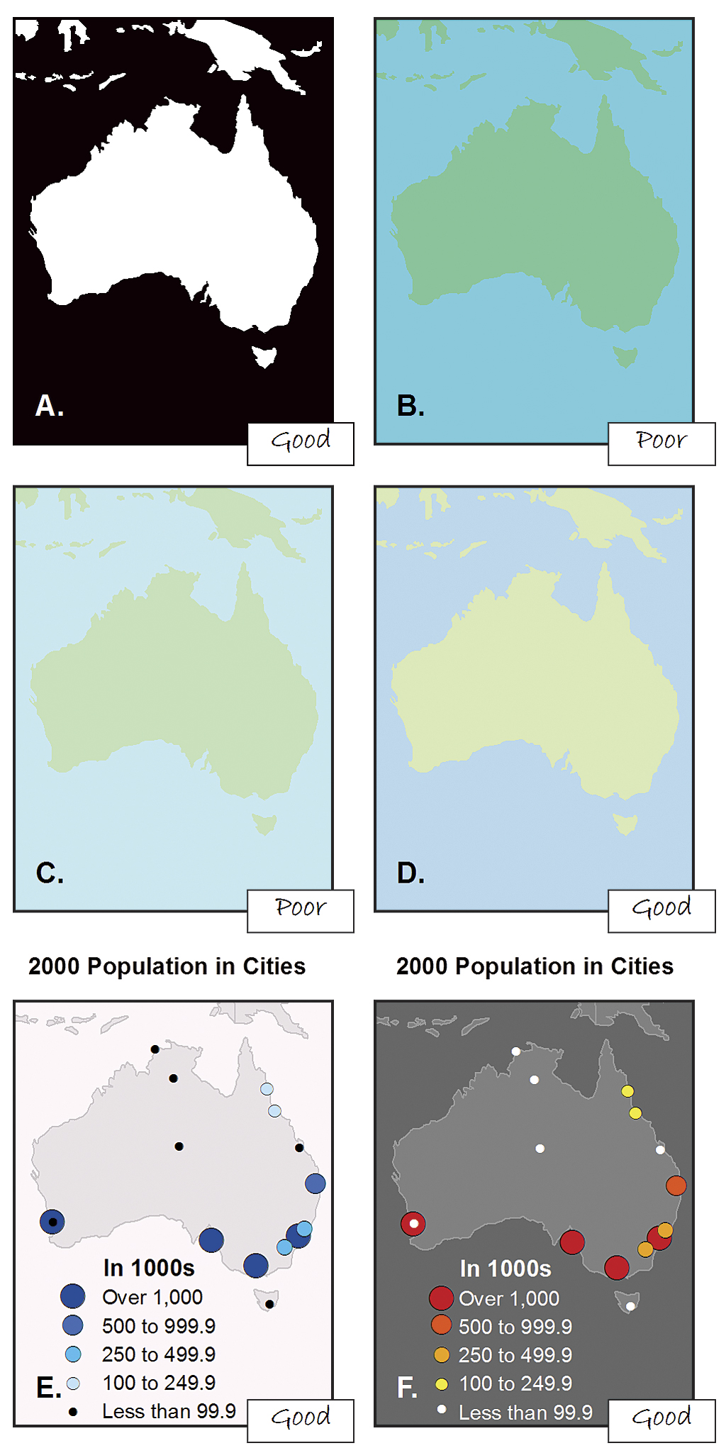
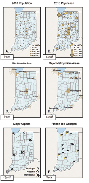
GeoSWG best practices for public health cartography:
These keep map products high-quality and consistent across a team.
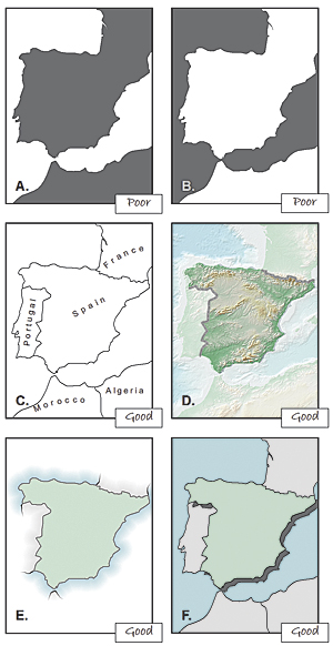
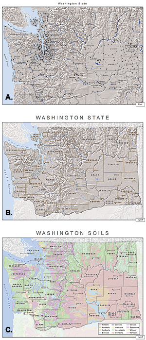
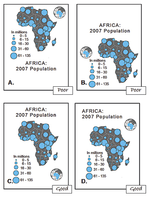
A thematic map in which values of a variable are encoded with a colour gradient.
viridis) and keep classes few (4 to 6).library(sf)
library(tidyverse)
library(here)
districts <- read_rds(here("spatial_files", "india_district_sf.rds"))
ggplot(districts) +
geom_sf(linewidth = 0.05, fill = "grey95", colour = "grey40") +
theme_void()
District polygons read with sf. Geometry plus attributes is all we need to start mapping.
districts |>                                  # an sf object
  left_join(indicator_df, by = "district") |> # attach the variable
  ggplot() +
  geom_sf(aes(fill = stunting), colour = "white", linewidth = 0.1) +
  scale_fill_viridis_c(option = "magma", direction = -1) +
  theme_void()
You build exactly this in Exercise 6 (NFHS stunting). The same recipe drives the maps in the rest of the module.
sf + ggplot2 recipe builds every map in the module.