Recreating John Snow’s map in R

Author

Your Name

Published

June 26, 2026

Load Packages

Load Data

Lets load the Snow.deaths data from the HistData package

snow_deaths <- HistData::Snow.deaths

snow_deaths |> class()
[1] "data.frame"
snow_deaths |> head()
  case         x         y
1    1 13.588010 11.095600
2    2  9.878124 12.559180
3    3 14.653980 10.180440
4    4 15.220570  9.993003
5    5 13.162650 12.963190
6    6 13.806170  8.889046

Let us now convert this data.frame into an sf object using the st_as_sf() function.

snow_deaths_sf <- snow_deaths |> 
  st_as_sf(coords = c('x', 'y'), crs = 4326)

Note the additional arguments such as coords and crs. Here we use the crs of 4326.

Let us now check the class of the newly created snow_deaths_sf object.

snow_deaths_sf |> class()
[1] "sf"         "data.frame"

Note that the sf object is also a data.frame.

Let us look at the structure of the sf object.

snow_deaths_sf
Simple feature collection with 578 features and 1 field
Geometry type: POINT
Dimension:     XY
Bounding box:  xmin: 8.280715 ymin: 6.090047 xmax: 17.93893 ymax: 16.97276
Geodetic CRS:  WGS 84
First 10 features:
   case                  geometry
1     1  POINT (13.58801 11.0956)
2     2 POINT (9.878124 12.55918)
3     3 POINT (14.65398 10.18044)
4     4 POINT (15.22057 9.993003)
5     5 POINT (13.16265 12.96319)
6     6 POINT (13.80617 8.889046)
7     7 POINT (13.10214 10.56081)
8     8 POINT (11.00403 11.86713)
9     9 POINT (15.15475 11.70451)
10   10 POINT (11.12639 9.643859)

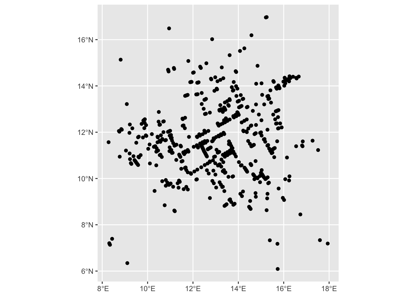
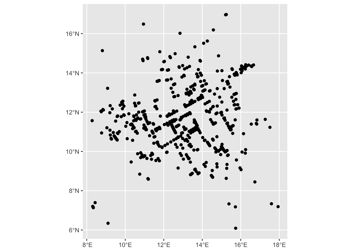
Let us now visualise the deaths using the geom_sf() function.

snow_deaths_sf |> 
  ggplot() +
  geom_sf() 

ggplot() +
  geom_sf(data = snow_deaths_sf)

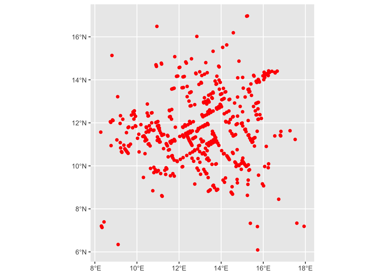
Let us now add color to the deaths using the color argument.

snow_deaths_sf |> 
  ggplot() +
  geom_sf(color = 'red') 

Now, we can add additional layers such as the water pumps and the streets of Soho, London.
snow_streets <- HistData::Snow.streets

snow_streets |> class()
[1] "data.frame"
snow_streets |> head()
  street n        x        y
1      1 2 16.73800 18.69600
2      1 2 17.66000 18.71200
3      2 2 14.46200 18.65500
4      2 2 16.73800 18.69600
5      3 2 12.79388 18.61613
6      3 2 14.46200 18.65500

We may have to convert the lat long coordinates into lines.

snow_streets_sf <- snow_streets |> 
  st_as_sf(coords = c('x', 'y'), crs = 4326) |> 
  group_by(street) |> 
  summarize(n = mean(n)) |> 
  st_cast('LINESTRING')

snow_streets_sf |> 
  slice(400:480)
Simple feature collection with 81 features and 2 fields
Geometry type: LINESTRING
Dimension:     XY
Bounding box:  xmin: 3.608146 ymin: 3.835 xmax: 19.88769 ymax: 7.997945
Geodetic CRS:  WGS 84
# A tibble: 81 × 3
   street     n                                                         geometry
    <int> <dbl>                                                 <LINESTRING [°]>
 1    400     2                           (12.38368 6.571151, 12.03881 7.088271)
 2    401     2                           (9.874142 6.963184, 9.169623 6.477379)
 3    402     2                            (8.591556 7.47125, 9.169623 6.477379)
 4    403     2                                (16.00062 6.598434, 14.981 6.473)
 5    404     6 (14.055 6.835, 14.981 6.473, 14.928 6.912, 14.83 7.03, 14.754 7…
 6    405     2                           (19.83346 6.469616, 19.79739 7.741153)
 7    406     2                           (19.83346 6.469616, 19.29552 7.436564)
 8    407     2                            (6.729623 6.96101, 5.854766 6.449976)
 9    408     2                           (10.19893 6.379891, 9.874142 6.963184)
10    409     2                           (8.980356 6.369051, 9.169623 6.477379)
# ℹ 71 more rows

Let us now look at the sf object.

snow_streets_sf
Simple feature collection with 528 features and 2 fields
Geometry type: LINESTRING
Dimension:     XY
Bounding box:  xmin: 3.39 ymin: 3.235 xmax: 19.912 ymax: 18.725
Geodetic CRS:  WGS 84
# A tibble: 528 × 3
   street     n                               geometry
    <int> <dbl>                       <LINESTRING [°]>
 1      1     2          (16.738 18.696, 17.66 18.712)
 2      2     2         (16.738 18.696, 14.462 18.655)
 3      3     2     (14.462 18.655, 12.79388 18.61613)
 4      4     2 (12.79388 18.61613, 11.59988 18.58831)
 5      5     2 (11.59988 18.58831, 10.97196 18.57368)
 6      6     2 (10.97196 18.57368, 10.79592 18.56957)
 7      7     2      (10.79592 18.56957, 8.533 18.524)
 8      8     2           (7.364 18.499, 8.533 18.524)
 9      9     2           (7.364 18.499, 6.703 18.485)
10     10     2      (6.478946 18.47905, 6.703 18.485)
# ℹ 518 more rows

Note the geometry type is now a sfc_LINESTRING.

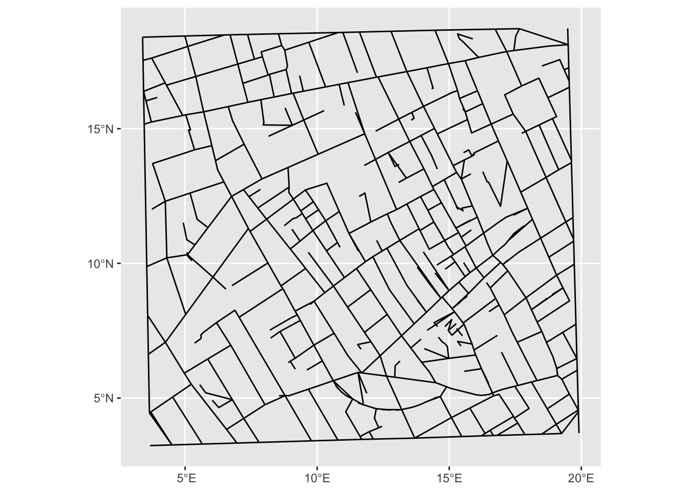
Let us plot the streets now.

snow_streets_sf |> 
  ggplot() + 
  geom_sf()

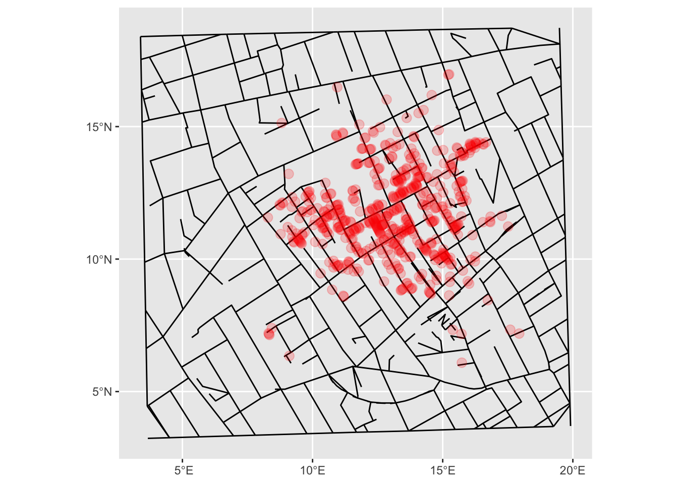
Let us add the streets of Soho, London as a new layer in our previously created deaths map.

ggplot() +
  geom_sf(data = snow_streets_sf) +
  geom_sf(data = snow_deaths_sf, color = 'red', alpha = 0.2, size = 3)

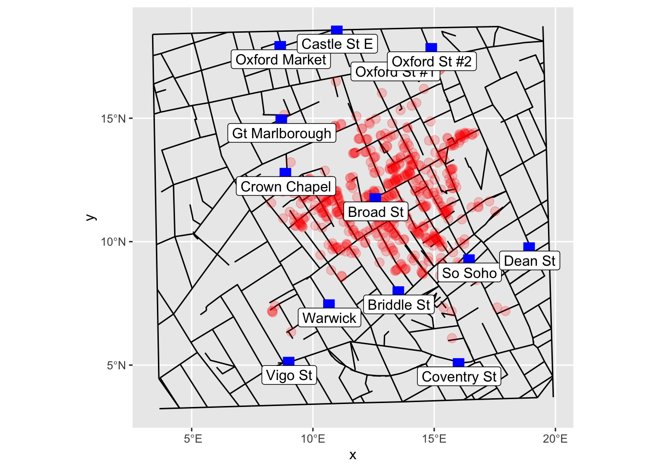
We can now add a new layer of water pumps on the above map.

snow_pumps_sf <- HistData::Snow.pumps |> 
  st_as_sf(coords = c('x', 'y'), crs = 4326)

ggplot() +
  geom_sf(data = snow_streets_sf) +
  geom_sf(data = snow_deaths_sf, color = 'red', alpha = 0.2, size = 3) +
  geom_sf(data = snow_pumps_sf , shape = 22, size = 4, fill = 'blue', color = 'blue')  +
  geom_sf_label(data = snow_pumps_sf, aes(label = label), nudge_x = 0.025, nudge_y = -0.5) # Add labels