Introduction to the
sf Package

Dr. Arun Mitra

Introduction

  • Objective: Learn the basics of the sf package in R for spatial data analysis.
  • Why sf?: Simplifies handling, analysis, and visualization of spatial data in R.

Overview of Spatial Data in R

  • Spatial Data: Data associated with locations in a geometric space.
  • Types:
    • Point data
    • Line data
    • Polygon data
  • Applications: Environmental monitoring, urban planning, epidemiology.

The sf Package

The sf package is an R implementation of Simple Features.

This package incorporates:

  • A new spatial data class system in R
  • Functions for reading and writing data
  • Tools for spatial operations on vectors

sf package
install.packages("sf")

Why the sf Package?

  • Integration: Seamlessly integrates with the tidyverse.
  • Efficiency: More efficient and user-friendly than previous spatial packages.
  • Standards: Adheres to international standards for spatial data.

sf package usage

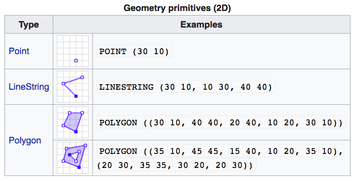
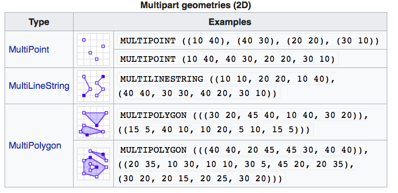
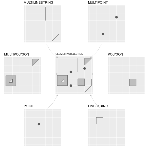
Geometry Types in sf

WKT Primitives WKT Multipart

sf Classes

Loading Spatial Data into R using sf

library(sf)
path_to_shape_file <- "path/to/shapefile.shp"
spatial_data <- st_read(path_to_shape_file)

Viewing the sf Object

print(spatial_data)

Plotting the sf Object

ggplot(spatial_data) +
  geom_sf()
ggplot(spatial_data) +
  geom_sf(aes(color = some_attribute))

Concept of the sf Package

  • Spatial Data Frame: Combines attributes and geometry.
  • Key Functions:
    • st_read(): Read spatial data.
    • st_write(): Write spatial data.
    • st_transform(): Transform coordinate systems.
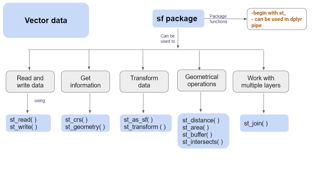
sf Concept Map

Dependencies of the sf Package
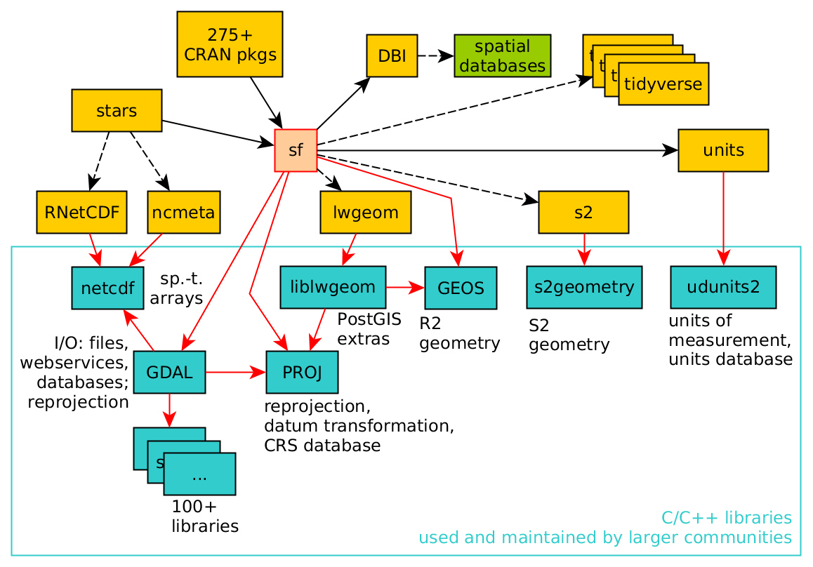
sf Dependencies

  • Key Dependencies:
    • GDAL: Geospatial Data Abstraction Library
    • PROJ: Cartographic Projections Library
    • GEOS: Geometry Engine

Methods in sf

methods(class="sf")
  • Common Methods:
    • st_union(): Union of geometries.
    • st_intersection(): Intersection of geometries.
    • st_buffer(): Buffer around geometries.

Interactive Mapping with sf

library(mapview)
mapview(spatial_data)

Practical Exercise: Loading and Plotting Data

  1. Load Data:
    • Use st_read() to load spatial data.
    • Example shapefile: "path/to/shapefile.shp"
  2. View Data:
    • Print the sf object.
  3. Plot Data:
    • Use ggplot2 to create a basic map.
library(sf)
spatial_data <- st_read("path/to/shapefile.shp")
print(spatial_data)
ggplot(spatial_data) + geom_sf()

Practical Exercise: Advanced Plotting

  1. Color by Attribute:
    • Use aes() to map colors to an attribute.
  2. Interactive Map:
    • Use mapview for interactive mapping.
ggplot(spatial_data) + geom_sf(aes(color = attribute))
library(mapview)
mapview(spatial_data)

Spatial Operations with sf

  • Buffering: Create buffer zones around geometries.
buffered <- st_buffer(spatial_data, dist = 100)
ggplot(buffered) + geom_sf()
  • Intersection: Find intersecting areas between geometries.
intersection <- st_intersection(spatial_data, another_spatial_layer)
ggplot(intersection) + geom_sf()

Spatial Joins with sf

  • Spatial Join: Combine attributes from different spatial datasets based on their spatial relationship.
joined_data <- st_join(spatial_data, another_spatial_layer)
ggplot(joined_data) + geom_sf()

Coordinate Transformations with sf

  • Transform Coordinates: Change the coordinate reference system (CRS) of spatial data.
transformed_data <- st_transform(spatial_data, crs = 4326)
ggplot(transformed_data) + geom_sf()

Where to Look for Help?
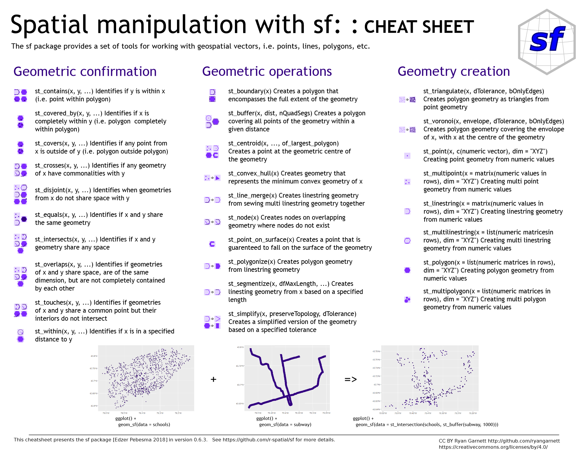
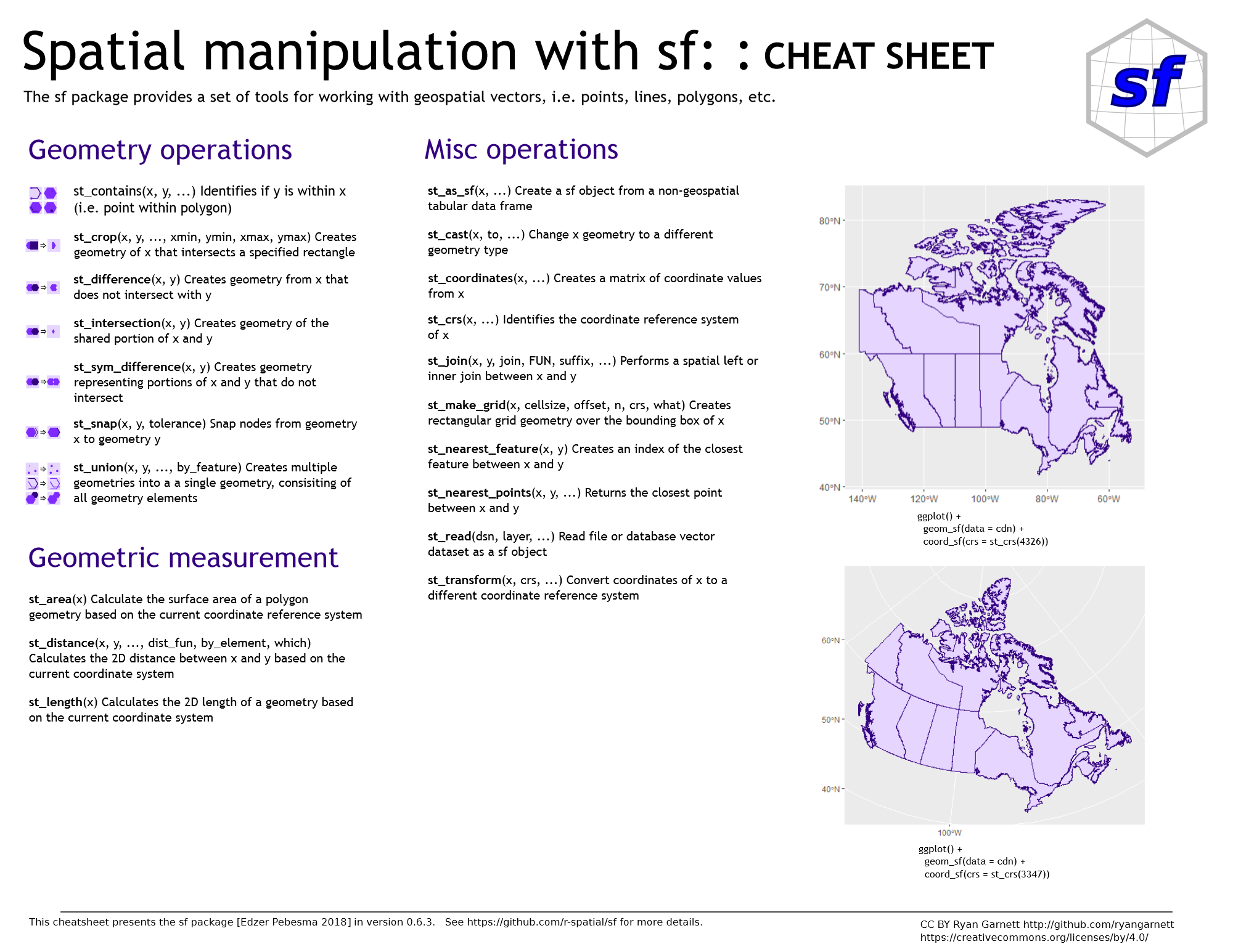
sf Cheatsheet 1

sf Cheatsheet 2

Questions

  • Any doubts or questions?
  • Hands-on practice time!